Example of Use#
[1]:
import powerplantmatching as pm
import pandas as pd
INFO:numexpr.utils:NumExpr defaulting to 8 threads.
ERROR 1: PROJ: proj_create_from_database: Open of /home/fabian/.miniconda3/share/proj failed
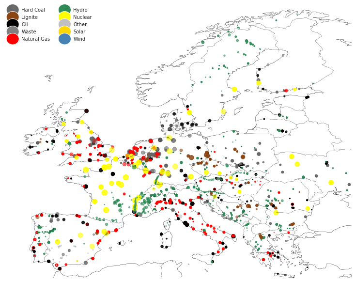
Load open source data published by the Global Energy Observatory, GEO. As you might know, this is not the original format of the database but the standardized format of powerplantmatching.
[2]:
geo = pm.data.GEO()

geo.head()
[2]:
| GEO | Name | Fueltype | Technology | Set | Country | Capacity | Efficiency | DateIn | DateRetrofit | DateOut | lat | lon | Duration | Volume_Mm3 | DamHeight_m | StorageCapacity_MWh | EIC | projectID |
|---|---|---|---|---|---|---|---|---|---|---|---|---|---|---|---|---|---|---|
| 0 | Duernrohr Chp | Hard Coal | CCGT | CHP | Austria | 373.384467 | NaN | 1985.0 | NaN | NaN | 48.3264 | 15.9246 | NaN | NaN | NaN | NaN | NaN | GEO-45151 |
| 1 | Duernrohr Chp | Hard Coal | CCGT | CHP | Austria | 324.521809 | NaN | 1985.0 | NaN | NaN | 48.3264 | 15.9246 | NaN | NaN | NaN | NaN | NaN | GEO-45151 |
| 2 | Mellach Chp | Hard Coal | Steam Turbine | CHP | Austria | 226.796491 | NaN | 1986.0 | NaN | NaN | 46.9115 | 15.4884 | NaN | NaN | NaN | NaN | NaN | GEO-45150 |
| 3 | Lenzing | Hard Coal | NaN | PP | Austria | 11.063243 | NaN | 1955.0 | NaN | NaN | 47.9767 | 13.6201 | NaN | NaN | NaN | NaN | NaN | GEO-45719 |
| 4 | Lenzing | Hard Coal | NaN | PP | Austria | 19.360676 | NaN | 1972.0 | NaN | NaN | 47.9767 | 13.6201 | NaN | NaN | NaN | NaN | NaN | GEO-45719 |
Load the data published by the ENTSOE which has the same format as the GEO data.
[3]:
entsoe = pm.data.ENTSOE()

entsoe.head()
[3]:
| ENTSOE | Name | Fueltype | Technology | Set | Country | Capacity | Efficiency | DateIn | DateRetrofit | DateOut | lat | lon | Duration | Volume_Mm3 | DamHeight_m | StorageCapacity_MWh | EIC | projectID |
|---|---|---|---|---|---|---|---|---|---|---|---|---|---|---|---|---|---|---|
| 0 | Aanekoski | Bioenergy | NaN | PP | Finland | 260.0 | NaN | NaN | NaN | NaN | NaN | NaN | NaN | NaN | NaN | NaN | 44W-T-YT-000017B | 44W-T-YT-000017B |
| 1 | Abono | Hard Coal | NaN | PP | Spain | 561.8 | NaN | NaN | NaN | NaN | NaN | NaN | NaN | NaN | NaN | NaN | 18WABO2-12345-0N | 18WABO2-12345-0N |
| 2 | Abono | Hard Coal | NaN | PP | Spain | 341.7 | NaN | NaN | NaN | NaN | NaN | NaN | NaN | NaN | NaN | NaN | 18WABO1-12345-0X | 18WABO1-12345-0X |
| 3 | Abthb | Hard Coal | NaN | PP | United Kingdom | 1590.0 | NaN | NaN | NaN | NaN | NaN | NaN | NaN | NaN | NaN | NaN | 48WSTN0000ABTHBN | 48WSTN0000ABTHBN |
| 4 | Abthgt | Oil | NaN | PP | United Kingdom | 51.0 | NaN | NaN | NaN | NaN | NaN | NaN | NaN | NaN | NaN | NaN | 48WSTN000ABTHGTK | 48WSTN000ABTHGTK |
Data Inspection#
Whereas various options of inspection are provided by the pandas package, some more powerplant-specific methods are applicable via an accessor ‘powerplant’. It gives you a convenient way to inspect, manipulate the data:
[4]:
geo.powerplant.plot_map(figsize=(11, 8));
[5]:
geo.powerplant.lookup().head(20).to_frame()
[5]:
| Capacity | ||
|---|---|---|
| Country | Fueltype | |
| Albania | Hydro | 1458.488 |
| Oil | 89.855 | |
| Austria | Hard Coal | 990.160 |
| Hydro | 7495.837 | |
| Natural Gas | 1112.211 | |
| Oil | 2935.705 | |
| Wind | 0.000 | |
| Belgium | Hard Coal | 1726.788 |
| Hydro | 1310.298 | |
| Natural Gas | 3034.023 | |
| Nuclear | 4966.076 | |
| Oil | 1093.076 | |
| Waste | 366.526 | |
| Wind | 0.000 | |
| Bosnia and Herzegovina | Hard Coal | 414.872 |
| Hydro | 2184.036 | |
| Lignite | 1226.446 | |
| Bulgaria | Hard Coal | 1742.461 |
| Hydro | 2457.894 | |
| Lignite | 2747.977 |
[6]:
geo.powerplant.fill_missing_commissioning_years().head()
/tmp/ipykernel_227814/846699350.py:1: DeprecatedWarning: fill_missing_commyears is deprecated as of 0.5.0 and will be removed in 0.6.0. This function was renamed to `fill_missing_commissioning_years`
  geo.powerplant.fill_missing_commyears().head()
[6]:
| GEO | Name | Fueltype | Technology | Set | Country | Capacity | Efficiency | DateIn | DateRetrofit | DateOut | lat | lon | Duration | Volume_Mm3 | DamHeight_m | StorageCapacity_MWh | EIC | projectID |
|---|---|---|---|---|---|---|---|---|---|---|---|---|---|---|---|---|---|---|
| 0 | Duernrohr Chp | Hard Coal | CCGT | CHP | Austria | 373.384467 | NaN | 1985 | 1985.0 | NaN | 48.3264 | 15.9246 | NaN | NaN | NaN | NaN | NaN | GEO-45151 |
| 1 | Duernrohr Chp | Hard Coal | CCGT | CHP | Austria | 324.521809 | NaN | 1985 | 1985.0 | NaN | 48.3264 | 15.9246 | NaN | NaN | NaN | NaN | NaN | GEO-45151 |
| 2 | Mellach Chp | Hard Coal | Steam Turbine | CHP | Austria | 226.796491 | NaN | 1986 | 1986.0 | NaN | 46.9115 | 15.4884 | NaN | NaN | NaN | NaN | NaN | GEO-45150 |
| 3 | Lenzing | Hard Coal | NaN | PP | Austria | 11.063243 | NaN | 1955 | 1955.0 | NaN | 47.9767 | 13.6201 | NaN | NaN | NaN | NaN | NaN | GEO-45719 |
| 4 | Lenzing | Hard Coal | NaN | PP | Austria | 19.360676 | NaN | 1972 | 1972.0 | NaN | 47.9767 | 13.6201 | NaN | NaN | NaN | NaN | NaN | GEO-45719 |
Of course the pandas functions are also very convenient:
[7]:
print('Total capacity of GEO is: \n  {} MW \n'.format(geo.Capacity.sum()));
print('The technology types are: \n {} '.format(geo.Technology.unique()))
Total capacity of GEO is:
  621580.8665191324 MW

The technology types are:
 ['CCGT' 'Steam Turbine' nan 'OCGT' 'Reservoir' 'Run-Of-River'
 'Pumped Storage' 'PV' 'CSP']
Incomplete data#
All open databases are so far not complete and cover only a part of overall European powerplants. We perceive the capacity gaps looking at the ENTSOE SO&AF Statistics.
[8]:
stats = pm.data.Capacity_stats()
[9]:
pm.plot.fueltype_totals_bar([geo, entsoe, stats], keys=["ENTSOE", "GEO", 'Statistics']);

The gaps for both datasets are unmistakable. Adding both datasets on top of each other would not be a solution, since the intersections of both sources are two high, and the resulting dataset would include many duplicates. A better approach is to merge the incomplete datasets together, respecting intersections and differences of each dataset.
Merging datasets#
Before comparing two lists of power plants, we need to make sure that the data sets are on the same level of aggregation. That is, we ensure that all power plant blocks are aggregated to power plant stations.
[10]:
dfs = [geo.powerplant.aggregate_units(), entsoe.powerplant.aggregate_units()]
intersection = pm.matching.combine_multiple_datasets(dfs)
INFO:powerplantmatching.cleaning:Aggregating blocks in data source 'GEO'.
INFO:powerplantmatching.cleaning:Aggregating blocks in data source 'ENTSOE'.
INFO:powerplantmatching.matching:Comparing data sources `GEO` and `ENTSOE`
[11]:
intersection.head()
[11]:
| GEO | Name | Fueltype | Technology | Set | Country | ... | Volume_Mm3 | DamHeight_m | StorageCapacity_MWh | EIC | projectID | ||||||||||
|---|---|---|---|---|---|---|---|---|---|---|---|---|---|---|---|---|---|---|---|---|---|
| GEO | ENTSOE | GEO | ENTSOE | GEO | ENTSOE | GEO | ENTSOE | GEO | ENTSOE | ... | GEO | ENTSOE | GEO | ENTSOE | GEO | ENTSOE | GEO | ENTSOE | GEO | ENTSOE | |
| 0 | Fierza Albania | Fierzag | Hydro | Hydro | Reservoir | Reservoir | PP | PP | Albania | Albania | ... | 0.0 | 0.0 | 0.0 | 0.0 | 0.0 | 0.0 | {nan, nan, nan, nan} | {54W-FIERZ000001A} | {GEO-42688} | {54W-FIERZ000001A} |
| 1 | Dalkia Poznan Karolin Chp | Karolin | Hard Coal | Hard Coal | NaN | NaN | CHP | PP | Poland | Poland | ... | 0.0 | 0.0 | 0.0 | 0.0 | 0.0 | 0.0 | {nan, nan, nan} | {19W0000000000725, 19W0000000000741} | {GEO-42494} | {19W0000000000725, 19W0000000000741} |
| 2 | Alqueva | Alqueva | Hydro | Hydro | Reservoir | Pumped Storage | PP | Store | Portugal | Portugal | ... | 0.0 | 0.0 | 0.0 | 0.0 | 0.0 | 0.0 | {nan, nan} | {16WALQUE-------F} | {GEO-43534} | {16WALQUE-------F} |
| 3 | Aguieira Brazil | Aguieira | Hydro | Hydro | Reservoir | Pumped Storage | PP | Store | Portugal | Portugal | ... | 0.0 | 0.0 | 0.0 | 0.0 | 0.0 | 0.0 | {nan, nan, nan} | {16WAGUIE-------3} | {GEO-43566} | {16WAGUIE-------3} |
| 4 | Zydowo | Zydowo | Hydro | Hydro | Pumped Storage | Pumped Storage | Store | Store | Poland | Poland | ... | 0.0 | 0.0 | 0.0 | 0.0 | 0.0 | 0.0 | {nan, nan, nan} | {19W0000000002426} | {GEO-42470} | {19W0000000002426} |
5 rows × 36 columns
The result of the matching process is a multi-indexed dataframe. To bring the matched dataframe into a convenient format, we combine the information of the two sources.
[12]:
intersection = intersection.powerplant.reduce_matched_dataframe()
intersection.head()
[12]:
| GEO | Name | Fueltype | Technology | Set | Country | Capacity | Efficiency | DateIn | DateRetrofit | DateOut | lat | lon | Duration | Volume_Mm3 | DamHeight_m | StorageCapacity_MWh | EIC | projectID |
|---|---|---|---|---|---|---|---|---|---|---|---|---|---|---|---|---|---|---|
| 0 | Fierzag | Hydro | Reservoir | PP | Albania | 500.0 | NaN | 1978.0 | 2003.0 | NaN | 42.251390 | 20.04306 | NaN | 0.0 | 0.0 | 0.0 | {54W-FIERZ000001A} | {'ENTSOE': {'54W-FIERZ000001A'}, 'GEO': {'GEO-... |
| 1 | Karolin | Hard Coal | NaN | CHP | Poland | 261.0 | NaN | 1985.0 | NaN | NaN | 52.436300 | 16.98790 | NaN | 0.0 | 0.0 | 0.0 | {19W0000000000725, 19W0000000000741} | {'ENTSOE': {'19W0000000000725', '19W0000000000... |
| 2 | Alqueva | Hydro | Pumped Storage | Store | Portugal | 508.0 | NaN | 2004.0 | NaN | NaN | 38.197500 | -7.49640 | NaN | 0.0 | 0.0 | 0.0 | {16WALQUE-------F} | {'ENTSOE': {'16WALQUE-------F'}, 'GEO': {'GEO-... |
| 3 | Aguieira | Hydro | Pumped Storage | Store | Portugal | 336.0 | NaN | 1981.0 | NaN | NaN | 40.340200 | -8.19700 | NaN | 0.0 | 0.0 | 0.0 | {16WAGUIE-------3} | {'ENTSOE': {'16WAGUIE-------3'}, 'GEO': {'GEO-... |
| 4 | Zydowo | Hydro | Pumped Storage | Store | Poland | 167.0 | NaN | 1971.0 | NaN | NaN | 54.024965 | 16.70690 | NaN | 0.0 | 0.0 | 0.0 | {19W0000000002426} | {'ENTSOE': {'19W0000000002426'}, 'GEO': {'GEO-... |
As you can see in the very last column, we can track which original data entries flew into the resulting one.
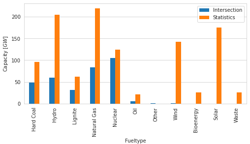
We can have a look into the Capacity statistics.
[13]:
pm.plot.fueltype_totals_bar([intersection, stats], keys=["Intersection", 'Statistics']);
[14]:
combined = intersection.powerplant.extend_by_non_matched(entsoe).powerplant.extend_by_non_matched(geo)
INFO:powerplantmatching.cleaning:Aggregating blocks in data source 'ENTSOE'.
INFO:powerplantmatching.cleaning:Aggregating blocks in data source 'GEO'.
[15]:
pm.plot.fueltype_totals_bar([combined, stats], keys=["Combined", 'Statistics']);
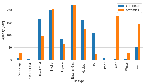
The aggregated capacities roughly match the SO&AF for all conventional powerplants.
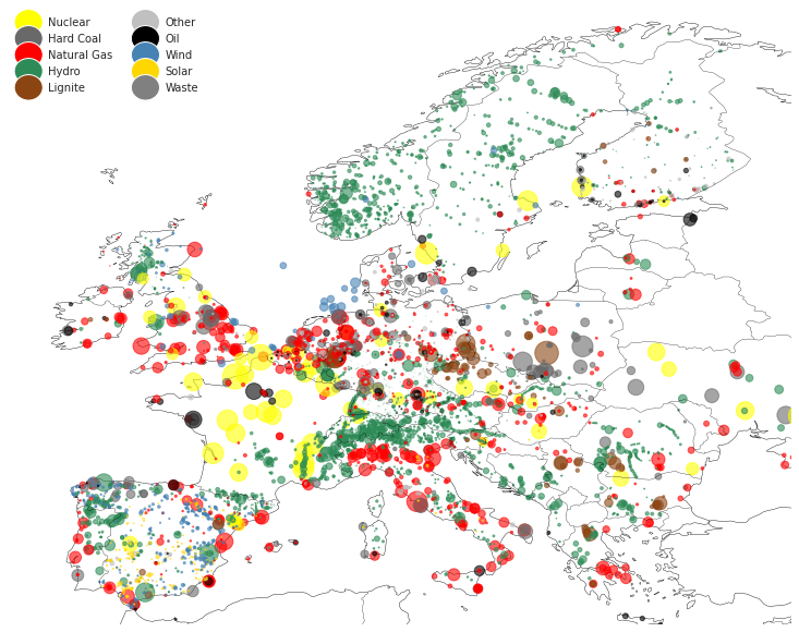
Processed Data#
powerplantmatching comes along with already matched data, this includes data from GEO, ENTSOE, OPSD, CARMA, GPD and ESE (ESE, only if you have followed the instructions).
[16]:
m = pm.collection.powerplants()
/tmp/ipykernel_227814/3660418824.py:1: DeprecatedWarning: matched_data is deprecated as of 5.5 and will be removed in 0.6. Use `powerplants` instead.
  m = pm.collection.matched_data()
[17]:
m.powerplant.plot_map(figsize=(11,8));
[18]:
pm.plot.fueltype_totals_bar([m, stats], keys=["Processed", 'Statistics']);
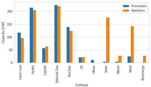
[19]:
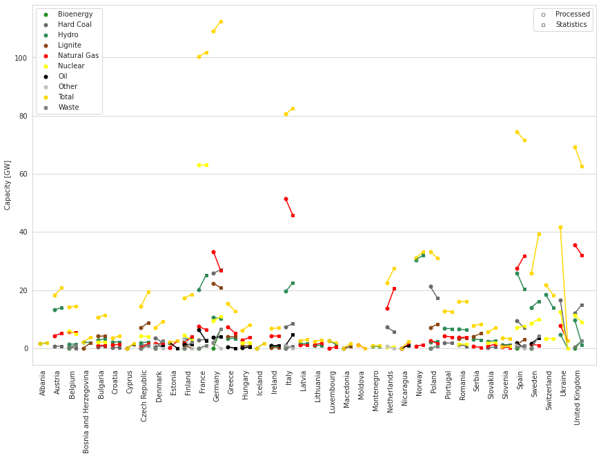
pm.plot.factor_comparison([m, stats], keys=['Processed', 'Statistics'])
/home/fabian/vres/py/powerplantmatching/powerplantmatching/plot.py:230: FutureWarning: The frame.append method is deprecated and will be removed from pandas in a future version. Use pandas.concat instead.
  compare.append(
[19]:
(<Figure size 864x648 with 1 Axes>, <AxesSubplot:ylabel='Capacity [GW]'>)
[20]:
m.head()
[20]:
| Matched Data | Name | Fueltype | Technology | Set | Country | Capacity | Efficiency | DateIn | DateRetrofit | DateOut | lat | lon | Duration | Volume_Mm3 | DamHeight_m | StorageCapacity_MWh | EIC | projectID |
|---|---|---|---|---|---|---|---|---|---|---|---|---|---|---|---|---|---|---|
| id | ||||||||||||||||||
| 0 | Emsland | Nuclear | Steam Turbine | CHP | Germany | 1336.000000 | 0.33 | 1988.0 | 1988.0 | 2022.0 | 52.481878 | 7.306658 | NaN | 0.0 | 0.0 | 0.0 | {'11WD7KKE-1K--KW5'} | {'ENTSOE': {'11WD7KKE-1K--KW5'}, 'OPSD': {'BNA... |
| 1 | Mellach | Hard Coal | Steam Turbine | CHP | Austria | 200.000000 | NaN | 1986.0 | 1986.0 | 2020.0 | 46.911700 | 15.488300 | NaN | 0.0 | 0.0 | 0.0 | {'14W-WML-KW-----0'} | {'BEYONDCOAL': {'BEYOND-AT-11'}, 'ENTSOE': {'1... |
| 2 | Eemshaven | Hard Coal | CCGT | PP | Netherlands | 1604.170304 | 0.58 | 2015.0 | NaN | 2029.0 | 53.440500 | 6.861200 | NaN | 0.0 | 0.0 | 0.0 | {'49W000000000044-'} | {'BEYONDCOAL': {'BEYOND-NL-12'}, 'ENTSOE': {'4... |
| 3 | Emile Huchet | Hard Coal | CCGT | PP | France | 596.493211 | NaN | 1958.0 | 2010.0 | 2022.0 | 49.152500 | 6.698100 | NaN | 0.0 | 0.0 | 0.0 | {'17W100P100P0345B', '17W100P100P0344D'} | {'BEYONDCOAL': {'BEYOND-FR-67'}, 'ENTSOE': {'1... |
| 4 | Fusina | Hard Coal | Steam Turbine | PP | Italy | 899.810470 | NaN | 1964.0 | NaN | 2025.0 | 45.431400 | 12.245800 | NaN | 0.0 | 0.0 | 0.0 | {'26WIMPI-S05FTSNK'} | {'BEYONDCOAL': {'BEYOND-IT-24'}, 'ENTSOE': {'2... |
[21]:
pd.concat([m[m.DateIn.notnull()].groupby('Fueltype').DateIn.count(),
          m[m.DateIn.isna()].fillna(1).groupby('Fueltype').DateIn.count()],
          keys=['DateIn existent', 'DateIn missing'], axis=1)
[21]:
| DateIn existent | DateIn missing | |
|---|---|---|
| Fueltype | ||
| Hard Coal | 191 | 10.0 |
| Hydro | 1743 | 1549.0 |
| Lignite | 98 | 9.0 |
| Natural Gas | 727 | 54.0 |
| Nuclear | 63 | NaN |
| Oil | 62 | 33.0 |
| Other | 103 | 75.0 |
| Solar | 12 | 191.0 |
| Waste | 84 | 17.0 |
| Wind | 220 | 163.0 |